
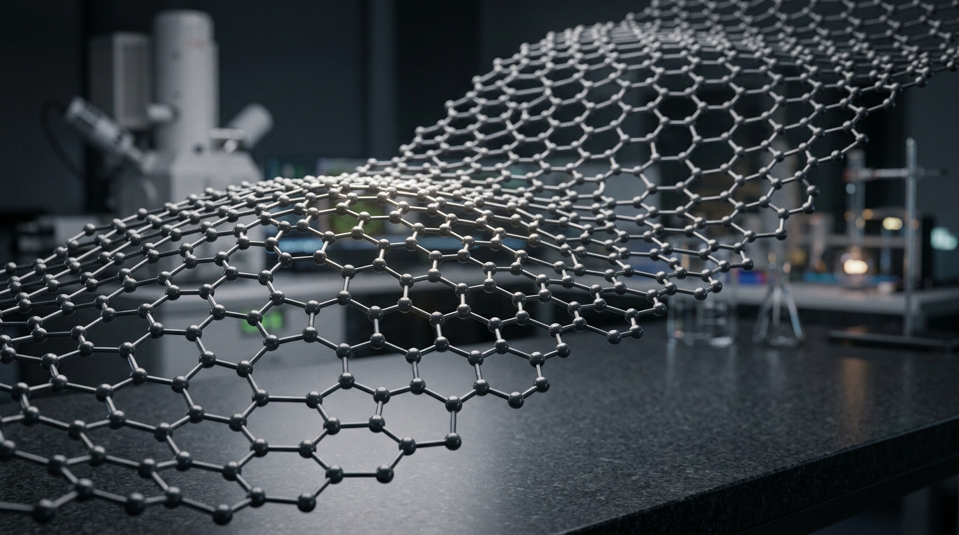
Graphene Structure
The graphene structure is a two-dimensional (2D) planar network of carbon atoms organized in a hexagonal, honeycomb crystal lattice. As a single atomic monolayer derived from bulk graphite, graphene represents the fundamental structural unit for several carbon allotropes, including fullerenes, carbon nanotubes, and graphite itself. Its distinct crystallographic geometry and quantum electronic configuration give rise to anomalous physical, mechanical, and electrical properties.
Lattice Geometry and Crystallography
At the crystallographic level, graphene is not a standard Bravais lattice on its own; rather, it is described as a triangular (hexagonal) Bravais lattice with a two-atom basis, traditionally labeled as sublattices A and B. Each carbon atom belonging to sublattice A is symmetrically coordinated with three equidistant nearest neighbors belonging to sublattice B, and vice versa.
The atomic arrangement is governed by well-defined geometric parameters:
- Carbon-Carbon Bond Length (a0): The interatomic distance between adjacent carbon atoms is approximately 0.142 nm (1.42 Å).
- Lattice Constant (a): The magnitude of the unit cell basis vectors is given by a = √3 · a0 ≈ 0.246 nm (2.46 Å).
- Lattice Vectors: In Cartesian coordinates, the primitive lattice vectors can be written as:
- a1 = (a/2) (√3, 1)
- a2 = (a/2) (√3, -1)
- Reciprocal Lattice and Brillouin Zone: The corresponding reciprocal lattice is also hexagonal. The first Brillouin zone is a regular hexagon whose corners are designated as the high-symmetry points K and K' (the Dirac points), with the zone center labeled as Γ and the edge midpoints labeled as M.
Because the two triangular sublattices are invariant under inversion only when mapped to each other, the spatial symmetry group of monolayer graphene is P6/mmm (point group D6h).
Orbital Hybridization and Chemical Bonding
The electronic configuration of an isolated ground-state carbon atom is 1s2 2s2 2p2. In the planar graphene lattice, the four valence electrons undergo sp2 hybridization, which splits the bonding landscape into two distinct electronic networks: in-plane σ-bonds and out-of-plane π-bonds.
In-Plane Sigma (σ) Bonds
The 2s, 2px, and 2py atomic orbitals mix to form three equivalent sp2 hybrid orbitals oriented at 120° angles within the 2D plane. These orbitals overlap covalently with adjacent carbon atoms to create strong σ-bonds. The σ-bonding state possesses a high binding energy and a localized electron density directly between the atomic nuclei. This dense, covalent scaffolding is responsible for the exceptional in-plane tensile strength, structural rigidity, and high structural stability of graphene.
Out-of-Plane Pi (π) Bonds
The remaining unhybridized 2pz orbital is oriented perpendicular to the atomic plane. The lateral overlap of these pz orbitals between neighboring carbon atoms forms a continuous, delocalized network of π (bonding) and π* (antibonding) bands that span across the entire sheet. Because the electrons in this conjugated system are free to move across the lattice, the π-network dictates graphene's electronic, optical, and high-frequency transport phenomena.
Electronic Band Structure and Dirac Fermions
The fundamental electronic behavior of pristine monolayer graphene is governed by its π-electron dispersion, conventionally modeled using a tight-binding Hamiltonian. Unlike conventional semiconductors or metals characterized by parabolic band curvature (where electron energy scales with the square of momentum, E ∝ k2), graphene exhibits a linear energy-momentum dispersion relation near the Fermi level.
Dirac Cones and Semimetallic Nature
The conduction band (π*) and valence band (π) meet continuously at six discrete points at the edges of the first Brillouin zone—specifically, at the two inequivalent sets of points, K and K'. These intersection points are termed Dirac points.
In the vicinity of these points, the energy spectrum forms conical surfaces known as Dirac cones, described by the relativistic-like equation:
E(q) = ± ħ vF |q|
Where q is the wavevector relative to the Dirac point, ħ is the reduced Planck constant, and vF is the Fermi velocity, which is roughly 106 m/s (approximately 1/300 the speed of light in a vacuum). Because the density of states vanishes precisely at the Fermi level in an undoped state, graphene behaves as a zero-bandgap semimetal (or zero-gap semiconductor). The charge carriers near the Dirac points behave effectively as massless relativistic particles (Dirac fermions), which eliminates backscattering from long-range impurities and supports high room-temperature charge carrier mobility.
Structural Hierarchy: Monolayer, Bilayer, and Few-Layer Graphene
The physical behavior of graphene changes when additional layers are stacked on top of the base monolayer. Interlayer coupling introduces modifications to the electronic band structure and vibrational modes.
Monolayer Graphene
A strictly single-atom-thick sheet (approximate mechanical thickness of ~0.335 nm). It features purely linear band dispersion, zero bandgap, and complete equivalence between its atomic sublattices within the plane.
Bilayer Graphene
Consists of two coupled graphene sheets. The most thermodynamically stable configuration is Bernal (AB) stacking, in which half of the carbon atoms in the upper layer sit directly above the carbon atoms of the lower layer, while the other half sit over the center of the underlying hexagonal rings. Bilayer graphene exhibits a parabolic band touching rather than linear dispersion. An applied external electric field perpendicular to the bilayer breaks inversion symmetry, enabling the opening of a tunable bandgap.
Few-Layer Graphene (FLG)
Comprises 3 to 10 distinct atomic layers. Stacking order can be Bernal (ABA) or Rhombohedral (ABC). As layer count increases, interlayer van der Waals interactions cause the electronic band structure to evolve rapidly toward that of bulk graphite, progressively screening external electrostatic fields.
Twisted Bilayer Graphene (Moiré Superlattices)
When two monolayer graphene sheets are stacked with an intentional rotational misalignment (twist angle θ), a long-period spatial interference pattern—a moiré superlattice—is formed. At specific configurations, notably the magic angle (θ ≈ 1.1°), the Fermi velocity drops toward zero, and isolated, topologically non-trivial flat bands emerge near the Fermi energy, giving rise to strongly correlated electron phenomena.
Defects in the Graphene Structure
While an idealized graphene lattice exhibits long-range crystalline order, synthetic graphene (such as that grown by chemical vapor deposition, or CVD) inherently contains structural imperfections that alter local electron transport, mechanical integrity, and chemical reactivity.
| Defect Category | Defect Type | Structural Description | Impact on Properties |
|---|---|---|---|
| 0D (Point Defects) | Single / Multiple Vacancies | Missing carbon atom(s) leaving unsaturated dangling bonds. | Local scattering center; decreases carrier mobility; increases chemical reactivity. |
| 0D (Point Defects) | Stone-Wales Defect | 90° rotation of a C-C bond turning four hexagons into two pentagons and two heptagons (5-7-7-5). | Preserves total atom count; locally distorts planarity; lowers mechanical failure threshold. |
| 1D (Line Defects) | Grain Boundaries | Stitched interfaces between misoriented crystalline domains containing periodic arrays of dislocations. | Scatters charge carriers; reduces thermal conductivity and macroscopic tensile strength. |
| 3D (Morphological) | Ripples and Wrinkles | Out-of-plane dynamic or static corrugations generated by thermal fluctuations or substrate mismatch. | Locally alters hybridization from pure sp2 toward mixed sp3; induces pseudomagnetic fields. |
Structure-Property Relationships
The macroscopic physical characteristics of graphene are direct consequences of its microscopic geometry and chemical bonding configuration:
- Mechanical Strength: The strong covalent sp2 σ-bonds generate an in-plane Young's modulus of approximately 1.0 TPa and an intrinsic tensile strength of ~130 GPa, making pristine graphene one of the strongest measured materials.
- Thermal Conductivity: In-plane heat transport is dominated by acoustic phonons traveling through the rigid, lightweight carbon lattice. Monolayer graphene exhibits thermal conductivity values ranging between 3,000 and 5,000 W/m·K at room temperature.
- Optical Transparency: Despite being only one atom thick, the universal optical absorption of monolayer graphene is governed purely by the fine-structure constant (πα ≈ 2.3%), resulting in an optical transmittance of 97.7% across the visible spectrum.
- Electrical Transport: The delocalized π-orbital overlap combined with linear dispersion at the Dirac points enables carrier mobilities exceeding 200,000 cm2/V·s at low temperatures in suspended or hexagonal boron nitride (h-BN) encapsulated configurations.
Structural Comparison with Other Carbon Allotropes
Carbon displays allotropic diversity based on hybridization states and structural dimensionality:
- Diamond (3D): Formed entirely by sp3 hybridization where each carbon atom is tetrahedrally bonded to four others. This creates an isotropic, non-conductive, ultra-hard insulator with a wide bandgap (~5.5 eV).
- Graphite (3D): Consists of parallel stacks of graphene monolayers held together by weak interlayer van der Waals forces, separated by an interlayer spacing of approximately 0.335 nm.
- Carbon Nanotubes (1D): Cylindrical structures formed by seamlessly rolling a graphene sheet along a specific chiral vector (n, m), exhibiting metallic or semiconducting behavior depending on rolling angle and diameter.
- Fullerenes (0D): Spherical, cage-like molecules (such as C60) consisting of hexagonal and pentagonal carbon rings that introduce curvature into an otherwise planar sp2 network.
Structural Characterization Methods
Analyzing the crystallographic quality and layer thickness of graphene samples requires high-resolution characterization techniques:
- Raman Spectroscopy: The primary non-destructive tool for evaluating graphene. It identifies layer count, strain, and defect density by analyzing the position, intensity, and shape of the characteristic G band (~1580 cm-1), the defect-activated D band (~1350 cm-1), and the second-order 2D band (~2680 cm-1).
- High-Resolution Transmission Electron Microscopy (HRTEM / STEM): Enables direct imaging of individual carbon atoms, atomic sublattices, point vacancies, and grain boundaries with sub-angstrom spatial resolution.
- Atomic Force Microscopy (AFM): Evaluates topography, surface roughness, and step heights to determine the precise layer count on supported substrates.